
You ran an A/B test. Variant B got more clicks than Variant A. But does that difference actually mean something, or did you just flip a lucky coin? That's the exact question A/B testing statistical significance answers, and getting it wrong means you'll make decisions based on noise instead of signal. At SocialRevver, where our entire content system runs on data-driven optimization loops, we've seen firsthand how misreading test results can send a content strategy sideways.
Statistical significance tells you whether the performance gap between two variants is real or random. Without it, you're guessing. And guessing doesn't scale. Whether you're testing hooks on short-form videos, subject lines on emails, or CTA placements on landing pages, you need a reliable method to separate actual wins from statistical flukes. The math behind it isn't as intimidating as it looks, but skipping it is expensive.
This article breaks down exactly how to calculate statistical significance for your A/B tests. You'll learn what p-values actually mean (and what they don't), how sample size affects your results, which formulas matter, and how to use free calculator tools to speed up the process. By the end, you'll have a clear framework for making confident, evidence-backed decisions instead of acting on gut feel dressed up as data.
Why statistical significance matters in A/B testing
Every test you run produces a result. The problem is that not every result tells the truth. Short-form video hooks, landing page layouts, email subject lines, all of these get tested constantly by marketers who then act on whatever number looks best. But a number that looks good after a 48-hour test with 200 visitors isn't necessarily telling you anything real. Statistical significance is the filter that separates a real performance difference from a result that could have happened by pure chance, and skipping that filter means you're basing real decisions on imaginary evidence.
The cost of acting on random results
When you declare a winner before your test reaches significance, you commit what statisticians call a false positive, or Type I error. You see Variant B outperform Variant A by 12%, you call it a win, you roll out the change across your funnel, and then conversions either stay flat or drop. That outcome isn't bad luck, it's predictable when you ignore the math. In a properly sized test, a 12% lift observed in the first few hundred sessions could easily fall within the normal variance of user behavior. You didn't find a winner. You found noise.
The downstream cost compounds fast. Every decision you build on a false positive becomes suspect. If you change your hook based on a statistically insignificant result and then optimize your CTA based on the new hook, you've stacked two unreliable decisions on top of each other. Your entire optimization process starts producing outputs that aren't grounded in reality. The longer this continues, the harder it becomes to diagnose why your content or funnel isn't performing the way your internal data suggests it should.
Decisions built on statistically insignificant results don't just waste time, they actively mislead your entire optimization process.
What significance actually protects you from
Understanding a b testing statistical significance is really about controlling two types of errors. A Type I error (false positive) means you think something works when it doesn't. A Type II error (false negative) means you miss a genuine improvement because your test lacked the power to detect it. Significance thresholds, set before you run the test, are the mechanism that controls your tolerance for both.
Beyond errors, significance also protects you from confirmation bias. When you run a test, you usually have a hypothesis, a version you believe will win. Without a significance threshold set in advance, you're more likely to stop a test early when the data happens to favor your hypothesis, and extend it when the data doesn't. This behavior is called peeking, and it artificially inflates your false positive rate. Setting a threshold upfront removes the temptation to stop whenever the result looks convenient.
Every change you deploy costs something, whether that's engineering time, creative production, or operational bandwidth. If you're shipping changes based on noise, you're consuming real resources to produce zero real improvement. Across dozens of tests per quarter, that waste adds up fast. Running tests with proper significance standards means every optimization you ship has a defensible, probability-based reason to exist. That's not just good science. It's how you build a content and conversion system you can actually trust.
The core concepts you must know
Before you can interpret any test result, you need a working understanding of the terms that make up the framework. A b testing statistical significance doesn't require a statistics degree, but it does require you to know exactly what each number represents and why it matters. These four concepts form the entire foundation of every test you'll ever run, and confusing any one of them will produce unreliable conclusions.
The null hypothesis and alternative hypothesis
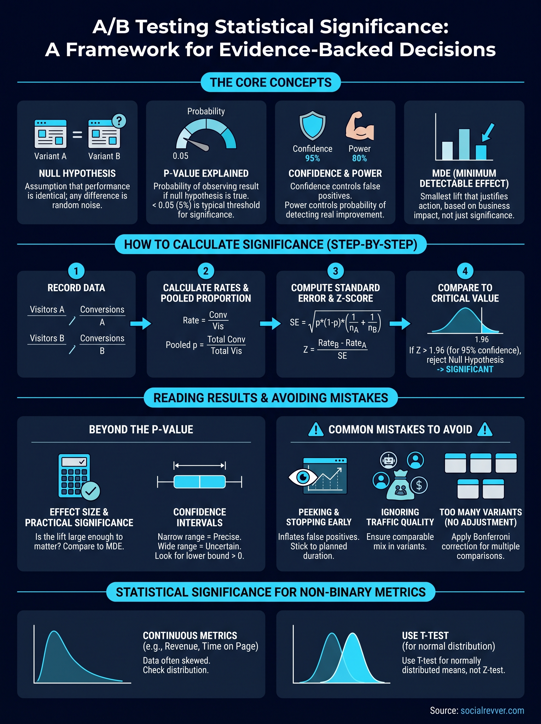
Every A/B test starts with a null hypothesis, which is the assumption that your two variants perform identically and that any observed difference is purely random. Your job during the test is not to prove your variant wins; it's to gather enough evidence to reject the null hypothesis. If you can reject it with enough confidence, the difference you observed is real, not coincidence.
The alternative hypothesis is simply the opposite claim: that a genuine difference exists between your variants. You never "prove" the alternative hypothesis; you only gather evidence strong enough to make the null hypothesis implausible. That distinction matters because it keeps you honest about what your results can and cannot confirm.
P-value explained
The p-value is the probability that you'd observe a result as extreme as the one you measured if the null hypothesis were actually true. A p-value below 0.05 means your result would occur by random chance less than 5% of the time, which is typically the threshold required to call a result significant. It does not tell you the size of the effect or guarantee that your variant will keep performing better at scale.
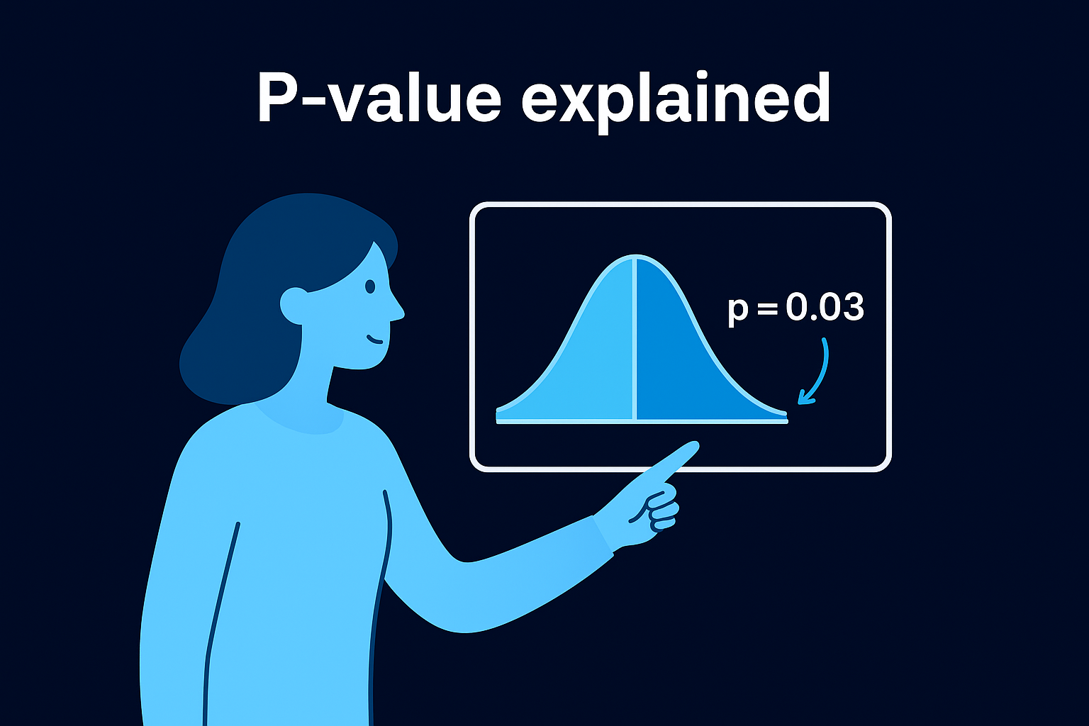
A p-value doesn't measure how confident you are that your variant wins; it measures how unlikely your result is under the assumption that nothing changed.
Many practitioners misread a p-value of 0.03 as "we're 97% sure this works," and that interpretation is incorrect and leads to overconfident shipping decisions.
Confidence level, power, and sample size
These three inputs control whether your test has any real capacity to detect a true difference. Confidence level is the inverse of your alpha threshold, so a 95% confidence level means you accept a 5% false positive rate. Statistical power, typically set at 80%, is the probability your test will catch a real improvement if one exists. Your minimum detectable effect (MDE) is the smallest lift that would actually matter to your business.
- Confidence level: usually 95%, higher for critical pages
- Statistical power: usually 80%, controls false negatives
- MDE: set based on business impact, not what looks impressive
- Sample size: calculated from all three inputs before you launch
Running a test without calculating required sample size in advance is the most common reason tests produce inconclusive results.
How to calculate significance step by step
Manual calculation makes the logic concrete. Even if you use a calculator tool for every real test, running through the math once by hand forces you to understand what the tool is actually measuring. The method below applies the two-proportion z-test, which is the standard approach for a b testing statistical significance when your metric is a conversion rate.
Step 1: Record your raw numbers
Start with four values: visitors in Variant A, conversions in Variant A, visitors in Variant B, and conversions in Variant B. Nothing else feeds into the calculation at this stage. As an example, say Variant A had 1,000 visitors and 50 conversions, while Variant B had 1,000 visitors and 65 conversions.
Step 2: Calculate each conversion rate and the pooled proportion
Divide conversions by visitors for each variant. Variant A converts at 5% (50/1,000) and Variant B converts at 6.5% (65/1,000). Then calculate the pooled proportion, which is the combined conversion rate across both variants:
- Pooled proportion (p): (50 + 65) / (1,000 + 1,000) = 0.0575
The pooled proportion represents what the conversion rate would look like if there were no difference between the two variants, which is exactly the assumption the null hypothesis makes.
Step 3: Compute the standard error and z-score
The standard error measures how much natural variation you'd expect between two groups of this size. Use this formula:

SE = sqrt(p * (1 - p) * (1/n_A + 1/n_B))
Plugging in the example values: SE = sqrt(0.0575 * 0.9425 * (1/1,000 + 1/1,000)) = approximately 0.01040.
Next, calculate the z-score by dividing the difference in conversion rates by the standard error:
Z = (0.065 - 0.05) / 0.01040 = approximately 1.44
Step 4: Compare your z-score to the critical value
For a 95% confidence level, the critical z-score is 1.96. If your z-score exceeds 1.96, you reject the null hypothesis and the result is statistically significant.
In this example, a z-score of 1.44 falls short of 1.96, which means you cannot call Variant B a winner yet, regardless of how promising the numbers look.
Your next move is to keep the test running until you accumulate enough data to push that z-score past the threshold, not to interpret the early numbers as directionally valid.
How to use a significance calculator correctly
Manual calculation builds understanding, but in practice, you'll use a significance calculator for every real test you run. The tools themselves are simple; the mistakes happen in how you use them. A calculator only produces a reliable result when you feed it accurate inputs and interpret the output within its actual limits. Treating the output number as a final verdict without understanding what it does and doesn't measure is where most practitioners go wrong.
What to input before you launch
Most free significance calculators ask for the same core inputs: visitors per variant, conversions per variant, your desired confidence level, and sometimes your statistical power. You should determine your confidence level and minimum detectable effect before the test starts, not after you see the results. Entering those parameters after the fact, once you already know which variant looks better, defeats the entire purpose of the framework. That approach lets your existing bias determine what threshold you apply, which makes the whole calculation meaningless.
The inputs also need to reflect your test as it actually ran. If you tested two variants but only measured a subset of your traffic, enter only the visitors who were actually exposed to the test. Mixing in organic traffic that was never part of the randomized experiment inflates your visitor count and makes your result look more significant than it is.
- Enter visitors, not sessions (one visitor can generate multiple sessions)
- Use raw conversion counts, not rates, if the tool allows it
- Set confidence level to 95% for standard tests and 99% for high-stakes pages
- Input statistical power at 80% unless you have a specific reason to adjust it
How to read the output correctly
A calculator will return a p-value, a confidence interval, and often a statement like "statistically significant at 95% confidence." What it will not tell you is whether the lift is large enough to matter for your business. A p-value of 0.02 on a conversion rate improvement of 0.1% is technically significant but commercially irrelevant. Reading a b testing statistical significance outputs correctly means pairing the significance result with an effect size check every single time.
Statistical significance tells you the result is real; it does not tell you the result is worth acting on.
Your confidence interval is the number that tells you the practical range of the true effect. If your calculator shows Variant B lifts conversions by 8% with a confidence interval of 0.5% to 15.5%, you have a wide range of uncertainty, and that width should factor directly into your deployment decision.
How to pick confidence, power, and MDE
These three parameters determine whether your test has enough rigor to produce a result worth trusting. Setting them after you've seen your data is the most reliable way to corrupt your test, because you'll unconsciously choose thresholds that validate the result you already observed. Every time you run a b testing statistical significance analysis, you need to lock these values in before you launch the test, not after.
Setting your confidence level
Your confidence level controls how much risk you're willing to accept for a false positive. The industry default is 95%, meaning you accept a 5% probability that a significant result occurred by chance. For standard content experiments, such as hook variations or thumbnail tests, 95% works well. For high-stakes decisions like changing a core checkout flow or repricing a product, raise that threshold to 99%. The tradeoff is that a higher confidence level requires a larger sample size to reach significance, so you need to account for that when you plan the test duration.
Raising your confidence threshold without adjusting your sample size estimate is one of the fastest ways to run an underpowered test.
Setting statistical power
Statistical power is the probability your test will actually detect a real difference if one exists. The standard setting is 80%, which means you accept a 20% chance of missing a genuine improvement. If you're running a test where missing a real winner would be costly, such as a major product page redesign, push your power to 90%. Like confidence level, higher power demands a larger sample size. Both parameters feed directly into your pre-test sample size calculation, so adjusting one without recalculating the other produces misleading results.
- 80% power: appropriate for routine content and copy tests
- 90% power: appropriate for high-revenue or high-traffic pages
- Never run a test without calculating the required sample size from your chosen power setting
Choosing your minimum detectable effect
Your MDE is the smallest lift that would actually justify acting on the result. Most practitioners make the mistake of setting their MDE as low as possible to keep sample size requirements manageable, but a 1% improvement in conversion rate might cost more to implement than it generates in revenue. Start by asking what lift would produce a measurable business outcome, then use that number. If your MDE is smaller than the natural daily variance in your conversion rate, your test will never produce a reliable result, regardless of how long you run it.
How to read results beyond significance
A significant p-value tells you one thing: the difference between your variants is unlikely to be random. It doesn't tell you whether that difference is large enough to matter, whether it holds across all your user segments, or how confident you should be in the exact size of the lift. Reading your results correctly means treating statistical significance as a starting point, not a finish line. Every solid analysis of a b testing statistical significance includes at least two additional checks after the p-value clears your threshold.
Effect size and practical significance
Effect size measures the magnitude of the difference, not just whether it exists. A test can reach 95% confidence on a 0.2% conversion rate improvement, but if implementing the winning variant requires two weeks of engineering work, that lift may not justify the cost. Before you ship any change, compare the measured lift against your pre-defined MDE. If the observed improvement falls at or below your MDE, the result is statistically significant but practically borderline, and you should factor that reality into your deployment decision rather than treating a green result as automatic approval to ship.
Statistical significance gives you permission to believe the result is real; effect size tells you whether acting on it is actually worth your time and resources.
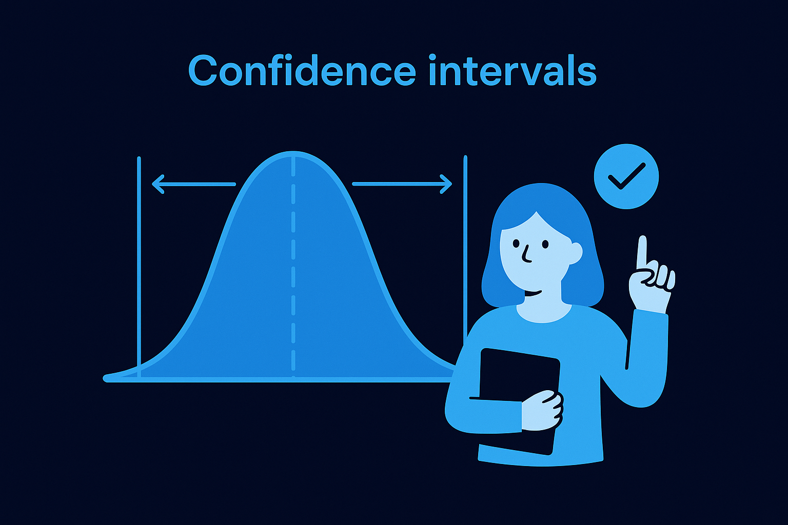
Confidence intervals as a decision tool
Your confidence interval gives you a range for where the true effect likely sits. A narrow interval, such as 4.5% to 5.5% lift, means your estimate is precise and reliable. A wide interval, such as 0.3% to 18.7% lift, tells you the test ran with too little data to pin down the true effect size, even if the result cleared your significance threshold. When the lower bound of your confidence interval falls near zero, treat the result with more caution before deploying it to your full audience. Confidence intervals are the most underused output in standard significance calculators, and ignoring them is how teams ship changes they later can't explain.
Segment-level breakdowns
A winning overall result can mask neutral or negative performance within specific user groups. After you confirm significance at the aggregate level, break your results down by device type, traffic source, and new versus returning visitors. A variant that performs better on desktop may actively hurt conversion on mobile. Running segment analysis after every significant test helps you deploy smarter, either by targeting the rollout to segments where the lift is genuine or by flagging an interaction effect that warrants a follow-up test. Skipping this step turns a reliable test result into a risky deployment.
Common mistakes that break your test
Most test failures don't come from bad hypotheses or weak variants. They come from procedural errors that corrupt the data before you ever calculate a result. Understanding where practitioners go wrong with a b testing statistical significance helps you avoid the traps that produce misleading outputs even when the math looks clean.
Peeking and stopping early
Checking your results mid-test and stopping when the numbers look favorable is called peeking, and it's the single most common way to inflate your false positive rate. Every time you look at live test results and consider stopping, you're effectively running an additional significance test. Each additional check raises the probability that a random fluctuation clears your threshold by coincidence. By the time you've checked ten times, your actual false positive rate can reach 30% or higher, even if your threshold is set at 5%.
Running one properly timed significance check at the end of a pre-planned test duration is the only way to keep your false positive rate at the level you actually set.
Lock in your planned test duration before launch based on your sample size calculation, then don't touch the results until that endpoint arrives.
Ignoring traffic quality and sample pollution
Your significance calculation is only as clean as the traffic you include. If your test runs across multiple traffic sources with different intent levels, such as paid search visitors mixed with organic social visitors, your conversion rates will shift based on traffic mix, not on your variant. That variance looks like noise to your significance test and forces you to collect far more data to reach a reliable conclusion. Segment your test traffic at setup so each variant receives a comparable mix of visitor types throughout the entire run.
Testing too many variants at once
Running three, four, or five variants simultaneously without adjusting your significance threshold for multiple comparisons creates what statisticians call the multiple comparisons problem. If you test five variants against a control at 95% confidence, your overall probability of at least one false positive across those comparisons climbs well above 5%. The correction for this is to use a Bonferroni adjustment, which divides your alpha threshold by the number of comparisons you're making. For two variants, this isn't an issue. For five or more, skipping the adjustment means your winning variant might just be the lucky noise in a crowded test, not a genuine improvement worth shipping.
- Two variants: no correction needed
- Three to five variants: apply Bonferroni correction
- Six or more variants: consider running sequential tests instead of simultaneous ones
Statistical significance for non-binary metrics
Most introductions to a b testing statistical significance use conversion rate as the example metric because it's binary: a visitor either converts or they don't. But many of the metrics that matter most to your business aren't binary. Revenue per visitor, average order value, time on page, and video watch time all produce continuous numerical data, and the two-proportion z-test you use for conversion rates doesn't apply to them. Running the wrong statistical test on the wrong type of data produces significance results that look valid but aren't, and shipping decisions based on that kind of error is no different from ignoring statistics entirely.
Testing continuous metrics like revenue per visitor
When your metric is continuous, the distribution of your data matters far more than it does with binary outcomes. Revenue per visitor, for example, is almost always heavily right-skewed because a small number of high-value purchases pull the average upward and inflate variance. That skew means the standard assumptions of a simple z-test break down. Before you run any significance test on a continuous metric, check whether your data follows a roughly normal distribution or whether outliers are compressing your ability to detect a real difference. For highly skewed distributions, you may need to log-transform your data or use a non-parametric test like the Mann-Whitney U test, which compares medians rather than means.
Applying a test designed for binary data to a continuous metric doesn't just reduce accuracy; it can flip your result entirely.
You also need to account for the fact that continuous metrics typically require larger sample sizes than binary metrics to reach significance at the same confidence level. Higher variance in your data means more noise, and more noise means you need more observations to detect the same size effect. Build that requirement into your pre-test sample size calculation before you launch.
Using the t-test for normally distributed outcomes
When your continuous metric is approximately normally distributed, the two-sample t-test is the standard tool for measuring statistical significance. It compares the means of two independent groups and accounts for the variance within each group. Most analytics platforms and significance calculators include a t-test option alongside the standard z-test, and selecting the right test is a one-step configuration change that makes a meaningful difference in result reliability. If you're evaluating a metric like average session duration or revenue per visitor on a large, well-distributed dataset, the t-test gives you a significance result you can actually trust and act on.
Next steps
You now have a complete framework for a b testing statistical significance: from the null hypothesis and p-value mechanics through manual z-score calculation, calculator use, and the right statistical test for continuous metrics. The most important move you can make right now is to apply the pre-test checklist before your next experiment, not after you've already collected data. Lock in your confidence level, statistical power, and minimum detectable effect upfront. Calculate your required sample size before you launch. Run one clean significance check at your pre-planned endpoint, then read the result alongside your confidence interval and segment breakdowns.
None of this complexity requires a statistics background, but it does require discipline in how you structure each test. If you want a content and optimization system that applies this kind of data rigor to every piece of short-form content you produce, apply to work with the SocialRevver team and get a free 40+ slide strategy built around your brand.